Introduction to reclues

Installation

You can install the development version from GitHub with:

# install.packages("devtools")
devtools::install_github("sciencificity/reclues")

Learn new skills while solving a mystery

The reclues package mimics the SQL Murder Mystery done by Northwestern’s Knight Lab - their game is set up to use SQL to solve the mystery, reclues makes their data available in R to solve the mystery using R ;-).

A brief of the task at hand is given in their walkthrough. Want to play the SQL version of the game online? Here it is courtesy of Simon Willison!

Getting Started: The Prompt (@knightlab)

Whodunnit??

A crime has taken place and the detective needs your help. The detective gave you the crime scene report, but you somehow lost it. You vaguely remember that the crime was a murder that occurred sometime on Jan.15, 2018 and that it took place in SQL City. All the clues to this mystery are buried in a huge database (DB), and you need to use your R skills to navigate through this vast network of information. Your first step to solving the mystery is to retrieve the corresponding crime scene report from the police department’s database.

Take a look at the cheatsheet (the Readme file or this Vignette) to learn some tips on how to do this using the tidyverse tools! From there, you can use your R skills to find the murderer. The crime may be solved with other tools besides tidy tools, please feel free to use the datasets as a learning tool for other packages in R or base R itself if that is your wish.

The data is available as individual dataframes:

crime_scene_report
drivers_license
facebook_event_checkin
get_fit_now_check_in
get_fit_now_member
income
interview
person

OR as the full SQLite database.

The cheatsheet is for tidyverse tools for now as a start, but since I am learning myself I may expand this to include data.table etc. in future. Have fun!

The datasets

These 8 datasets will be available as soon as you install the package. Here is a brief description of what each dataset contains. Use ? combined with the dataset name to get the help page for the dataset (e.g. ?crime_scene_report).

Table Name	Fields	Rows
crime_scene_report	date, type, description, city	1,228 rows
drivers_license	id, age, height, eye_color, hair_color, gender, plate_number, car_make, car_model	10,007 rows
facebook_event_checkin	person_id, event_id, event_name, date	20,011 rows
get_fit_now_check_in	membership_id, check_in_date, check_in_time, check_out_time	2,703 rows
get_fit_now_member	id, person_id, name, membership_start_date, membership_status	184 rows
income	ssn, annual_income	7,514 rows
interview	person_id, transcript	4,991 rows
person	id, name, license_id, address_number, address_street_name, ssn	10,011 rows

SQLite DB

The raw SQLite database as per @knightlab is also available through the get_db() function. To use the SQLite DB for your investigation you will need the DBI package.

install.packages("DBI")

Some useful functions to view the data

If you are using the dataframes `crime_scene_report`, `person` etc.

library(reclues)
library(dplyr)
# see the first 6 observations
head(crime_scene_report)
#> # A tibble: 6 x 4
#>       date type    description                                      city   
#>      <int> <chr>   <chr>                                            <chr>  
#> 1 20180115 robbery A Man Dressed as Spider-Man Is on a Robbery Spr~ NYC    
#> 2 20180115 murder  Life? Dont talk to me about life.                Albany 
#> 3 20180115 murder  Mama, I killed a man, put a gun against his hea~ Reno   
#> 4 20180215 murder  REDACTED REDACTED REDACTED                       SQL Ci~
#> 5 20180215 murder  Someone killed the guard! He took an arrow to t~ SQL Ci~
#> 6 20180115 theft   Big Bully stole my lunch money!                  Chicago

# pivots data with column names (features) running down the page,
# and a few of the values of the data listed for each feature.
tibble::glimpse(drivers_license)
#> Observations: 10,007
#> Variables: 9
#> $ id           <int> 100280, 100460, 101029, 101198, 101255, 101494, 1...
#> $ age          <int> 72, 63, 62, 43, 18, 48, 53, 57, 40, 81, 87, 78, 5...
#> $ height       <int> 57, 72, 74, 54, 79, 55, 78, 70, 65, 58, 67, 81, 5...
#> $ eye_color    <chr> "brown", "brown", "green", "amber", "blue", "blue...
#> $ hair_color   <chr> "red", "brown", "green", "brown", "grey", "red", ...
#> $ gender       <chr> "male", "female", "female", "female", "female", "...
#> $ plate_number <chr> "P24L4U", "XF02T6", "VKY5KR", "Y5NZ08", "5162Z1",...
#> $ car_make     <chr> "Acura", "Cadillac", "Scion", "Nissan", "Lexus", ...
#> $ car_model    <chr> "MDX", "SRX", "xB", "Rogue", "GS", "Sportage", "9...

# Another nifty function is skimr::skim(dataset_name), the %>% is called a pipe
# and comes from the magrittr package. It essentially says take the dataset `get_fit_now_member`
# and sends it to the skimr::skim() function as the first input.
# Note how it tells you the number of "categories" in character data types - this can help understand
# which of your variables are categories vs free text strings - here membership_status 
# looks like a category, while id and name look like free text.
get_fit_now_member %>% skimr::skim()
#> Skim summary statistics
#>  n obs: 184 
#>  n variables: 5 
#> 
#> -- Variable type:character ---------------------------------------------------------------
#>           variable missing complete   n min max empty n_unique
#>                 id       0      184 184   5   5     0      184
#>  membership_status       0      184 184   4   7     0        3
#>               name       0      184 184   9  20     0      184
#> 
#> -- Variable type:integer -----------------------------------------------------------------
#>               variable missing complete   n     mean       sd    p0
#>  membership_start_date       0      184 184 2e+07     4312.73 2e+07
#>              person_id       0      184 184 54898.17 27272.12 10319
#>       p25     p50     p75  p100     hist
#>  2e+07    2e+07   2e+07   2e+07 <U+2581><U+2581><U+2581><U+2582><U+2587><U+2581><U+2581><U+2583>
#>  31197.75 55806.5 79230.5 99602 <U+2587><U+2586><U+2583><U+2587><U+2586><U+2586><U+2587><U+2586>

SELECT

In R dplyr’s select() works much the same as SELECT in SQL. You use it to get only specific columns you are interested in.

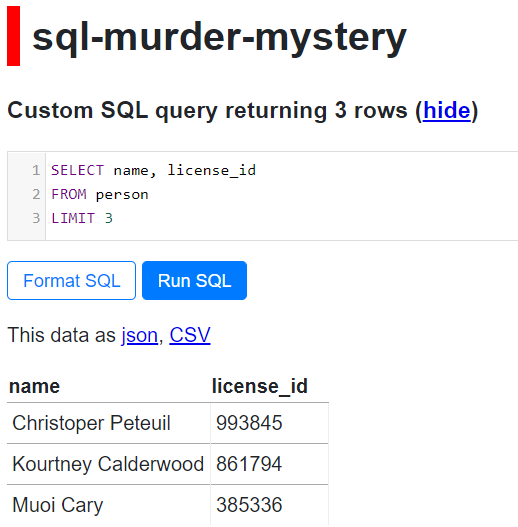
Let’s say I wanted a closer look at the name and license_id of a person.

# Let's have a look at a few columns of interest from the drivers_license table
person %>% 
  dplyr::select(name, license_id) %>% 
  head(3) %>% 
  # formattable func from the formattable package just prints a nice table in the Readme
  formattable::formattable()

name	license_id
Christoper Peteuil	993845
Kourtney Calderwood	861794
Muoi Cary	385336

SQL Equivalent is:

SELECT name, license_id
FROM person
LIMIT 3

Here’s a snippet from the online SQL version:

SELECT Helpers in `dplyr`

Or maybe I want the car related columns from the drivers_license table? dplyr has some handy helper functions that can assist us! By the way, I don’t know of a SQL function that can give us this - if you do please drop me a line!

# There are also helper functions to select columns of interest
# starts_with('start_text') will help select columns that begin with start_text
# ends_with('end_text') will help select columns that end with end_text
drivers_license %>% 
  # Maybe I am only interested in the columns describing the car...
  dplyr::select(starts_with('car')) %>% 
  head(3) %>% 
  # formattable just prints a nice table in the Readme
  formattable::formattable()

car_make	car_model
Acura	MDX
Cadillac	SRX
Scion	xB

LIMIT

Let’s say we wanted to see a part of the data - the head() function returns 6 observations and performs a similar functionality as the LIMIT keyword in SQL.

head() gives you the first 6 observations of the data in the “table”
tail() gives you the last 6 observations of the data in the “table”

You can also specify a number as an argument to the head() or tail() functions. For example, head(15) and tail(10) will give you the first 15, and last 10 observations respectively.

crime_scene_report %>% 
  dplyr::select(description) %>% 
  head(8) %>% 
  # formattable func from the formattable package just prints a nice table in the Readme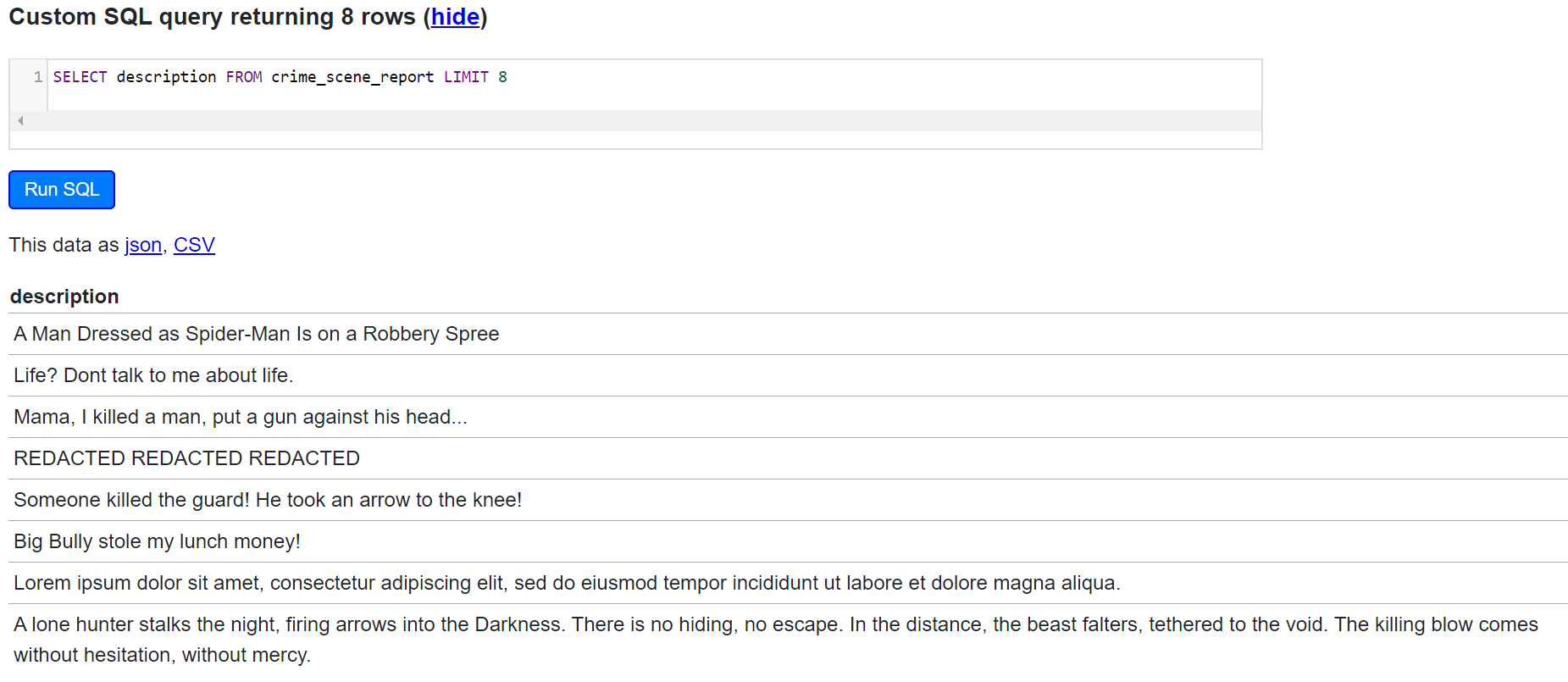
  formattable::formattable()

description
A Man Dressed as Spider-Man Is on a Robbery Spree
Life? Dont talk to me about life.
Mama, I killed a man, put a gun against his head…
REDACTED REDACTED REDACTED
Someone killed the guard! He took an arrow to the knee!
Big Bully stole my lunch money!
Lorem ipsum dolor sit amet, consectetur adipiscing elit, sed do eiusmod tempor incididunt ut labore et dolore magna aliqua.
A lone hunter stalks the night, firing arrows into the Darkness. There is no hiding, no escape. In the distance, the beast falters, tethered to the void. The killing blow comes without hesitation, without mercy.

SQL Equivalent is:

SELECT description FROM crime_scene_report LIMIT 8

Here’s a snippet from the online SQL version:

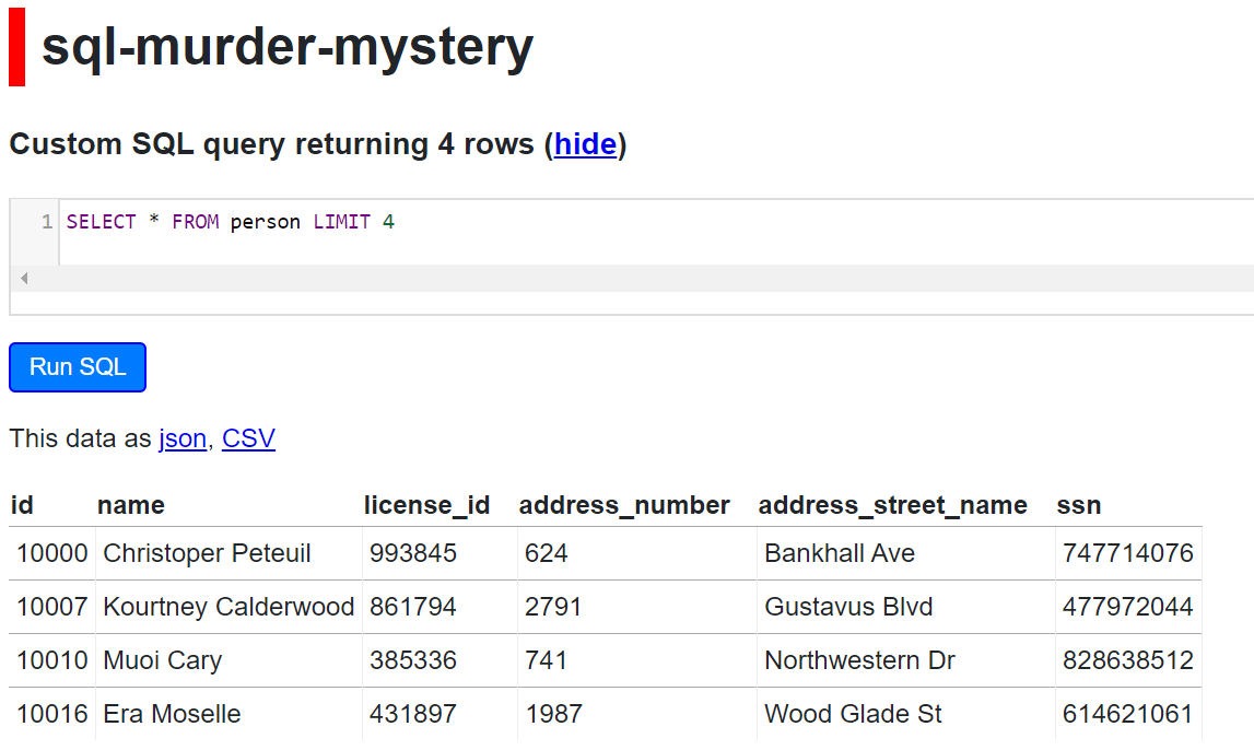
Maybe I am interested in having a look at all variables associated with a person but I just want to have a look at the data not bring back all 10,011 rows.

person %>% 
  head(4) %>% 
  formattable::formattable()

id	name	license_id	address_number	address_street_name	ssn
10000	Christoper Peteuil	993845	624	Bankhall Ave	747714076
10007	Kourtney Calderwood	861794	2791	Gustavus Blvd	477972044
10010	Muoi Cary	385336	741	Northwestern Dr	828638512
10016	Era Moselle	431897	1987	Wood Glade St	614621061

SQL Equivalent is:

SELECT * FROM person LIMIT 4;

Here’s a snippet from the online SQL version:

DISTINCT

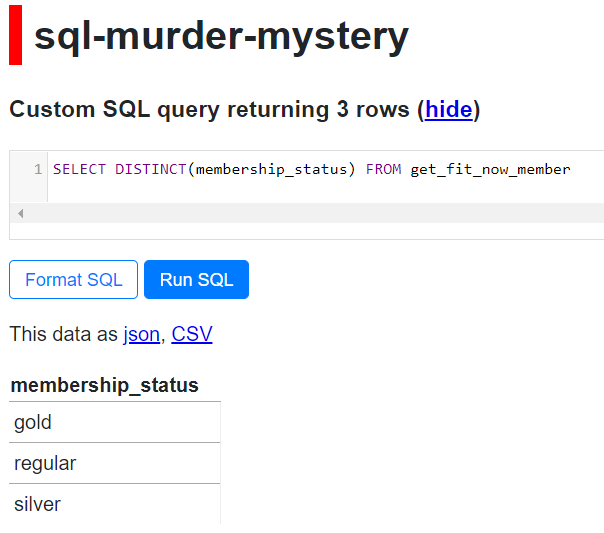
Let’s say we wanted to see the different kinds of membership statuses.
The membership_status field in the Get Fit Now Membership table seems to contain this info. We will use the distinct function from dplyr.

library(magrittr)

# T he magrittr package contains the pipe %>% function. Take the Get Fit Now membership data AND THEN
# give me the distinct values for the `membership_status` variable.
get_fit_now_member %>% 
    dplyr::distinct(membership_status) %>% 
    formattable::formattable()

membership_status
gold
regular
silver

SQL Equivalent is:

SELECT DISTINCT(membership_status) FROM get_fit_now_member

Here’s a snippet from the online SQL version:

COUNT DISTINCT

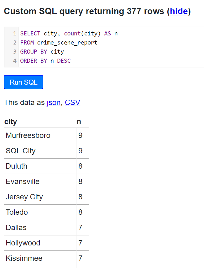
Let’s say we were wondering which city has the highest number of crimes - here we want the city and a count of the times that city is mentioned in the crime scene report …

crime_scene_report %>% 
    dplyr::count(city) %>% 
    dplyr::arrange(desc(n)) %>% 
    # filter to limit the print-out
    dplyr::filter(n >= 7) %>% 
    formattable::formattable()

city	n
Murfreesboro	9
SQL City	9
Duluth	8
Evansville	8
Jersey City	8
Toledo	8
Dallas	7
Hollywood	7
Kissimmee	7
Lancaster	7
Little Rock	7
Newark	7
Portsmouth	7
Reno	7
Waterbury	7
Wilmington	7

Hhmmm looks like SQL City is quite notorious for crime!

SQL Equivalent is:

SELECT city, count(city) AS n
FROM crime_scene_report
GROUP BY city
ORDER BY n DESC

Here’s a snippet from the online SQL version:

Magnify long pieces of text

Sometimes there are fields like crime_scene_report.description which are hard to see because the text runs over several lines. Even using View() or printing just the description to the screen sometimes does not help.

Enter pull() from the dplyr package which extracts a column from the data.

Hint: You will need something like this to read some of the textual description and transcript information.

crime_scene_report %>% 
  head(8) %>% 
  dplyr::pull(description) %>% 
  # these next 2 lines are just for displaying the result nicely in the Readme
  tibble::enframe(name = NULL) %>% 
  formattable::formattable()

value
A Man Dressed as Spider-Man Is on a Robbery Spree
Life? Dont talk to me about life.
Mama, I killed a man, put a gun against his head…
REDACTED REDACTED REDACTED
Someone killed the guard! He took an arrow to the knee!
Big Bully stole my lunch money!
Lorem ipsum dolor sit amet, consectetur adipiscing elit, sed do eiusmod tempor incididunt ut labore et dolore magna aliqua.
A lone hunter stalks the night, firing arrows into the Darkness. There is no hiding, no escape. In the distance, the beast falters, tethered to the void. The killing blow comes without hesitation, without mercy.

interview %>% 
  filter(stringr::str_length(transcript) >= 230) %>% 
  dplyr::pull(transcript) %>% 
  # these next 2 lines are just for displaying the result nicely in the Readme
  tibble::enframe(name = NULL) %>% 
  formattable::formattable()

value
I was hired by a woman with a lot of money. I don’t know her name but I know she’s around 5’5" (65“) or 5’7” (67"). She has red hair and she drives a Tesla Model S. I know that she attended the SQL Symphony Concert 3 times in December 2017.

LIKE

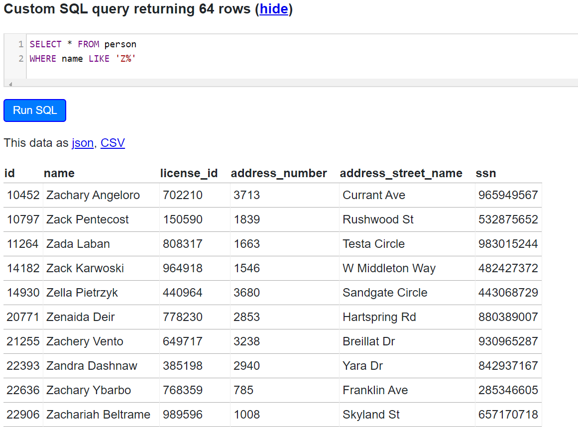
Let’s say we’re interested in finding the people that start with a Z. We will use the stringr package for this. The str_detect() function can be used in conjunction with regular expressions - here we looking for names that start with (^) Z.

library(stringr)
person %>% 
  dplyr::filter(stringr::str_detect(name, "^Z")) %>% 
  # Limit to top 5 for the print-out
  head(5) %>% 
  formattable::formattable()

id	name	license_id	address_number	address_street_name	ssn
10452	Zachary Angeloro	702210	3713	Currant Ave	965949567
10797	Zack Pentecost	150590	1839	Rushwood St	532875652
11264	Zada Laban	808317	1663	Testa Circle	983015244
14182	Zack Karwoski	964918	1546	W Middleton Way	482427372
14930	Zella Pietrzyk	440964	3680	Sandgate Circle	443068729

SQL Equivalent is:

SELECT * FROM person
WHERE name LIKE ‘Z%’

Here’s a snippet from the online SQL version:

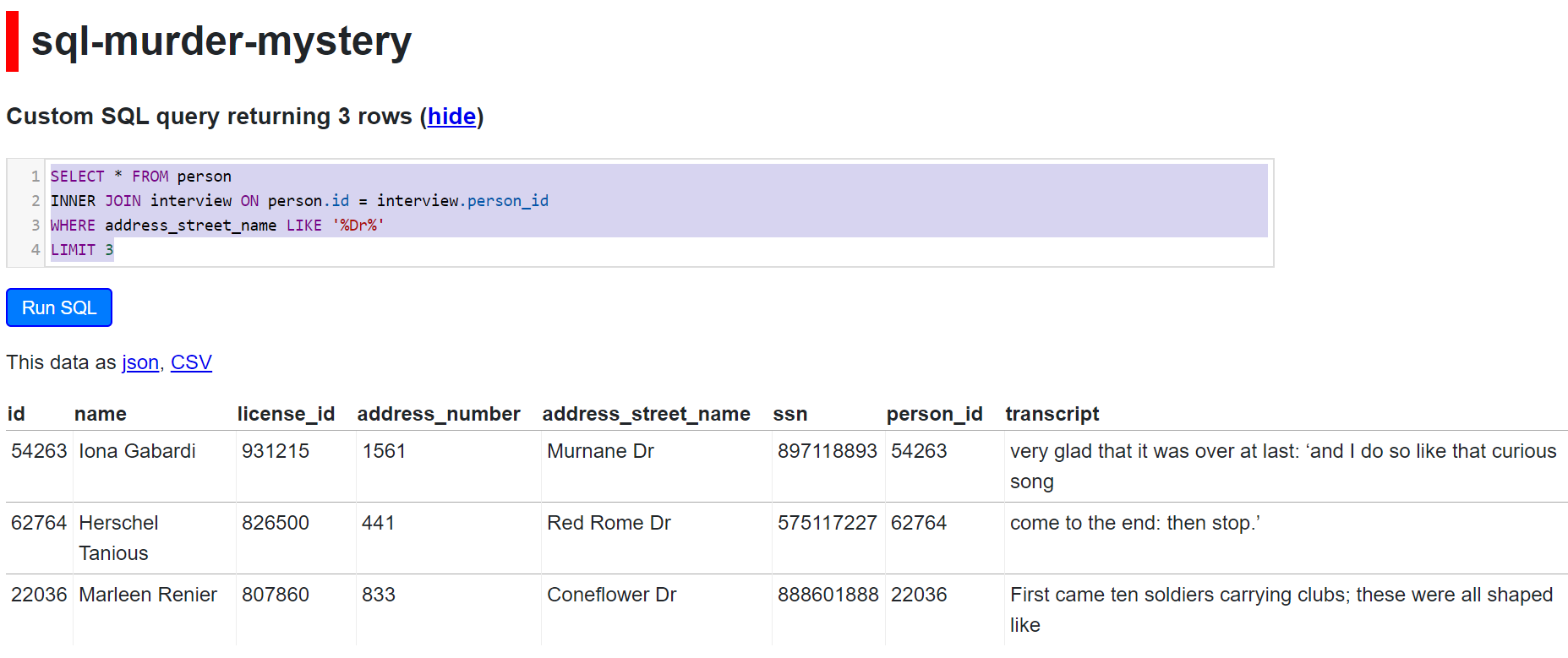
JOINS

dplyr has joining functions such as inner_join(), left_join() etc. for joining one table to another. This mimics the SQL INNER JOIN etc.
You will notice that the person table has a field called id and the interview table has a person_id field. Let’s join these tables and see what we get.

person %>% 
  # Since the two tables have diff field names for the common field
  # we have to specify the `by` argument.
  # by = c('field_name_from_left_table' = 'field_name_from_right_table')
  dplyr::inner_join(interview, by = c('id' = 'person_id')) %>% 
  # Let's say we're only interested in interviews from people who live
  # on some Drive abbreviated to 'Dr'
  dplyr::filter(stringr::str_detect(address_street_name, 'Dr')) %>% 
  # Limit for print-out
  head(3) %>% 
  formattable::formattable()

id	name	license_id	address_number	address_street_name	ssn	transcript
10027	Antione Godbolt	439509	2431	Zelham Dr	491650087	nearer to watch them, and just as she came up to them she heard one of
10034	Kyra Buen	920494	1873	Sleigh Dr	332497972	a kind of serpent, that’s all I can say.’
10039	Francesco Agundez	278151	736	Buswell Dr	861079251	Beau–ootiful Soo–oop!

SELECT * FROM person
INNER JOIN interview ON person.id = interview.person_id
WHERE address_street_name LIKE ‘%Dr%’
LIMIT 3

Here’s a snippet from the online SQL version:

Some useful funtions for DB Manipulation

If you are using the SQLite DB

To work with the murder mystery SQLite database we’ll first have to make a connection to it. The DBI::dbConnect() is usually used to set up the connection to the database, however in this package calling the get_db() function does the work for you.

library(DBI)
library(dbplyr)

# Retrieve a connection to the SQLite database embedded in this package
conn <- get_db()

We can list the tables of the database by using the the DBI::dbListTables() as below. It is basically saying “Hey, what tables are there in this database I’ve connected to?”.

# List the tables in the database
DBI::dbListTables(conn)
#> [1] "crime_scene_report"     "drivers_license"       
#> [3] "facebook_event_checkin" "get_fit_now_check_in"  
#> [5] "get_fit_now_member"     "income"                
#> [7] "interview"              "person"                
#> [9] "solution"

We may connect through the connection we created to get an idea of what any one of the tables contains. Here we look at the crime_scene_report table. The function below says “What’s the crime_scene_report table like? Show me the first few rows, please.”

SQL Equivalent is:

SELECT * FROM crime_scene_report LIMIT 10;

# Let's glimpse the data in crime_scene_report table 
dplyr::tbl(conn, "crime_scene_report")
#> # Source:   table<crime_scene_report> [?? x 4]
#> # Database: sqlite 3.29.0
#> #   [C:\Users\vebashini\AppData\Local\Temp\Rtmpi0R3pJ\temp_libpath4647c3c2f19\reclues\db\sql-murder-mystery.db]
#>        date type    description                                      city  
#>       <int> <chr>   <chr>                                            <chr> 
#>  1 20180115 robbery A Man Dressed as Spider-Man Is on a Robbery Spr~ NYC   
#>  2 20180115 murder  Life? Dont talk to me about life.                Albany
#>  3 20180115 murder  Mama, I killed a man, put a gun against his hea~ Reno  
#>  4 20180215 murder  REDACTED REDACTED REDACTED                       SQL C~
#>  5 20180215 murder  Someone killed the guard! He took an arrow to t~ SQL C~
#>  6 20180115 theft   Big Bully stole my lunch money!                  Chica~
#>  7 20180115 fraud   "Lorem ipsum dolor sit amet, consectetur adipis~ Seatt~
#>  8 20170712 theft   "A lone hunter stalks the night, firing arrows ~ SQL C~
#>  9 20170820 arson   "Wield the Hammer of Sol with honor, Titan, it ~ SQL C~
#> 10 20171110 robbery "The Gjallarhorn shoulder-mounted rocket system~ SQL C~
#> # ... with more rows

Notice how the rows are marked as ?? in the output table<crime_scene_report> [?? x 4]. The source is a SQLite database and it just returns a taste of the data and does not bring the entire table back into R, hence it has no idea how many rows there are in the crime_scene_report table embedded in the sql-murder-mystery database.

In an R Markdown file you can use the connection to directly bring back data like writing a SQL Query at an SQL editor using the {sql, connection = conn} code block - please remove the "" around the code block if running in a markdown file.

“{sql, connection = conn} SELECT * FROM person LIMIT 3”

-- Direct SQL on the DB through the connection
SELECT * 
FROM person
LIMIT 3

3 records
id	name	license_id	address_number	address_street_name	ssn
10000	Christoper Peteuil	993845	624	Bankhall Ave	747714076
10007	Kourtney Calderwood	861794	2791	Gustavus Blvd	477972044
10010	Muoi Cary	385336	741	Northwestern Dr	828638512

dbplyr

show_query() to Learn SQL!

dbplyr helps take dplyr code and convert it into SQL queries which then get run on the database you connected to. Here we’ll have a look at a few of the commands. The show_query() function from dplyr allows you to see the generated SQL - this is a handy way to learn SQL as well!

Also check out the documentation and vignette of dbplyr to learn more.

tbl(conn, "crime_scene_report") %>% 
  filter(type == "murder") %>% 
  show_query()
#> <SQL>
#> SELECT *
#> FROM `crime_scene_report`
#> WHERE (`type` = 'murder')

tbl(conn, "drivers_license") %>% 
  count(eye_color) %>% 
  show_query()
#> <SQL>
#> SELECT `eye_color`, COUNT() AS `n`
#> FROM `drivers_license`
#> GROUP BY `eye_color`

Execute query on a database - but use dplyr like coding!

tbl(conn, "crime_scene_report") %>% 
  filter(type == "murder") 
#> # Source:   lazy query [?? x 4]
#> # Database: sqlite 3.29.0
#> #   [C:\Users\vebashini\AppData\Local\Temp\Rtmpi0R3pJ\temp_libpath4647c3c2f19\reclues\db\sql-murder-mystery.db]
#>        date type  description                                   city       
#>       <int> <chr> <chr>                                         <chr>      
#>  1 20180115 murd~ Life? Dont talk to me about life.             Albany     
#>  2 20180115 murd~ Mama, I killed a man, put a gun against his ~ Reno       
#>  3 20180215 murd~ REDACTED REDACTED REDACTED                    SQL City   
#>  4 20180215 murd~ Someone killed the guard! He took an arrow t~ SQL City   
#>  5 20170107 murd~ "‘It proves nothing of the sort!’ said Alice~ Memphis    
#>  6 20170108 murd~ "get” is the same thing as “I get what I lik~ Round Lake~
#>  7 20170108 murd~ "       HEARTHRUG,\n"                         Jacksonvil~
#>  8 20170111 murd~ "\n"                                          Springdale 
#>  9 20170121 murd~ "her, to pass away the time.\n"               Murfreesbo~
#> 10 20170122 murd~ "came near her, she began, in a low, timid v~ Temecula   
#> # ... with more rows

tbl(conn, "drivers_license") %>% 
  count(eye_color) 
#> # Source:   lazy query [?? x 2]
#> # Database: sqlite 3.29.0
#> #   [C:\Users\vebashini\AppData\Local\Temp\Rtmpi0R3pJ\temp_libpath4647c3c2f19\reclues\db\sql-murder-mystery.db]
#>   eye_color     n
#>   <chr>     <int>
#> 1 amber      1947
#> 2 black      2017
#> 3 blue       2025
#> 4 brown      2030
#> 5 green      1988

Like

We can use the %LIKE% functionality here to get data. Let’s say we’re looking for an individual named “Zelda” …

tbl(conn, "person") %>% 
  filter(name %LIKE% 'Zel%')
#> # Source:   lazy query [?? x 6]
#> # Database: sqlite 3.29.0
#> #   [C:\Users\vebashini\AppData\Local\Temp\Rtmpi0R3pJ\temp_libpath4647c3c2f19\reclues\db\sql-murder-mystery.db]
#>      id name          license_id address_number address_street_na~      ssn
#>   <int> <chr>              <int>          <int> <chr>                 <int>
#> 1 14930 Zella Pietrz~     440964           3680 Sandgate Circle      4.43e8
#> 2 47936 Zelda Kitten      391768           3469 E Marie Blvd         9.97e8
#> 3 61047 Zella Binegar     360327           2955 Blake Rd             2.14e8
#> 4 75261 Zelda Oney        455975           1674 Miramount Rd         1.97e8
#> 5 87530 Zelma Feery       178807           2116 Eglinton Dr          8.75e8
#> 6 93766 Zelda Ang         558785           2313 Thorncroft Way       2.91e8

#> <SQL>
#> SELECT *
#> FROM `person`
#> WHERE (`name` LIKE 'Zel%')

Think you solved it

Run the following commands in R once you think you’ve solved the problem. You will need the DBI package and if you’ve been using the datasets to solve the mystery and not the SQLite database (i.e. the individual dataframes of person, drivers_license etc.) then uncomment the first line to make a connection to the database, run the queries below after you’ve put in the culprit you suspect, and then disconnect from the database.

conn <- reclues::get_db()

# Replace 'Insert the name of the person you found here' with the name of the individual you found.
DBI::dbExecute(conn, "INSERT INTO solution VALUES (1, 'Insert the name of the person you found here')")

# Did we solve it? You'll either get a "That's not the right person." or a "Congrats,..." message.
DBI::dbGetQuery(conn, "SELECT value FROM solution;")

DBI::dbDisconnect(conn)

Resources

SQL

Brandon Rohrer (@_brohrer_) has a curated list of resources here

R

Hadley Wickham and Garrett Grolemund’s book R for Data Science
dplyr cheatsheet
dplyr video and another here
stringr
Primers
RStudio Education
Jumpstart with R
Cheatsheets
Loads of other resources
For DB interaction via R using dbplyr.

Installation

Learn new skills while solving a mystery

Getting Started: The Prompt (@knightlab)

Whodunnit??

The datasets

SQLite DB

Some useful functions to view the data

If you are using the dataframes crime_scene_report, person etc.

SELECT

SELECT Helpers in dplyr

LIMIT

DISTINCT

COUNT DISTINCT

Magnify long pieces of text

LIKE

JOINS

Some useful funtions for DB Manipulation

If you are using the SQLite DB

dbplyr

show_query() to Learn SQL!

Execute query on a database - but use dplyr like coding!

Like

Think you solved it

Resources

SQL

R

Contents

If you are using the dataframes `crime_scene_report`, `person` etc.

SELECT Helpers in `dplyr`